Classification

Learning Outcomes

  • K-Nearest Neighbors

  • Bayes’ Classifier

  • Linear and Quadratic Discriminant Analysis

  • Naive Bayes

Setup

Code
import pandas as pd
from palmerpenguins import load_penguins
from plotnine import *
from sklearn.discriminant_analysis import LinearDiscriminantAnalysis
from sklearn.naive_bayes import GaussianNB
from sklearn.discriminant_analysis import QuadraticDiscriminantAnalysis

Classification

The practice of classifying data points into different categories.

K-Nearest Neighbors

K-Nearest Neighbors

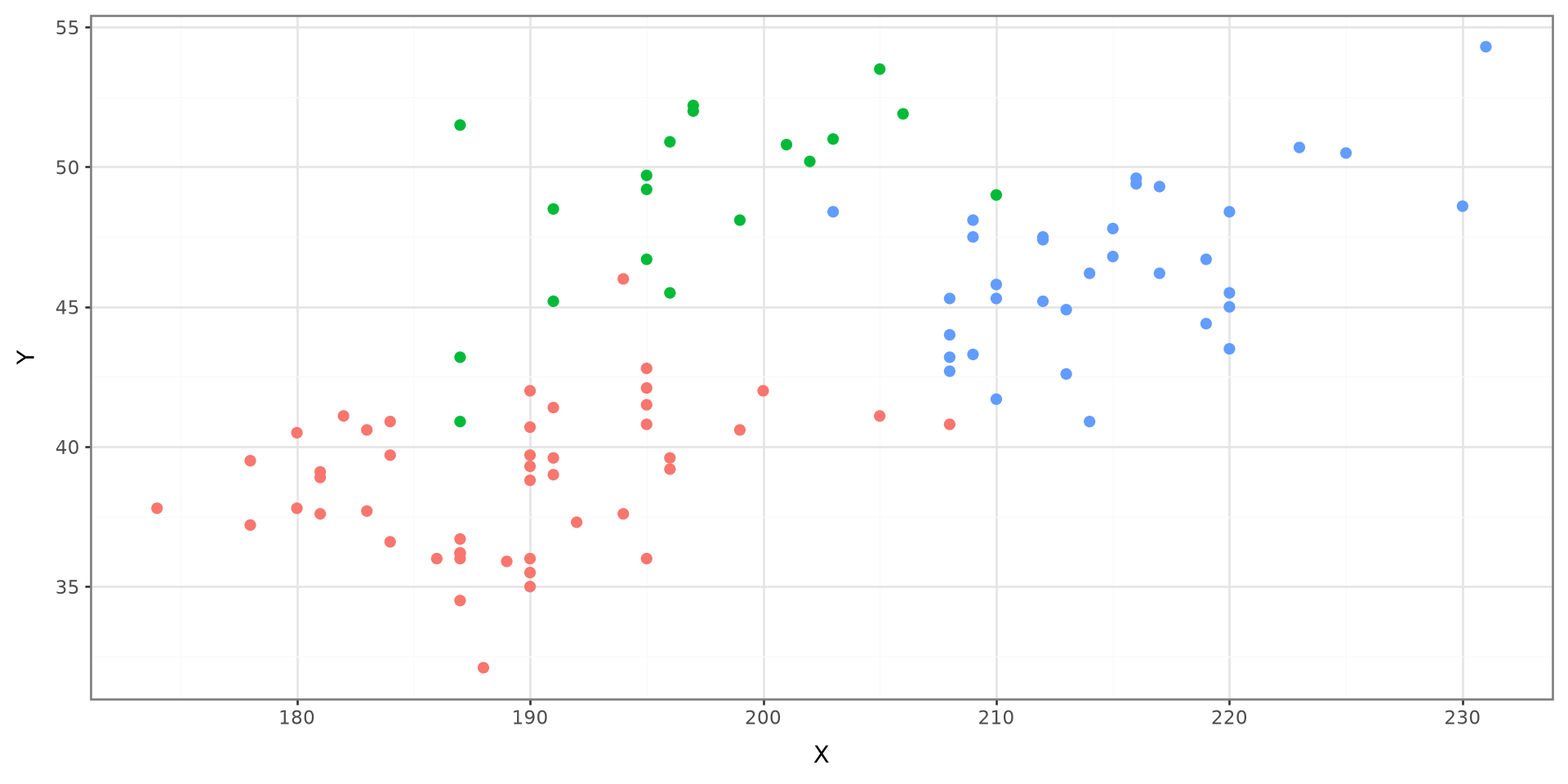
K-Nearest Neighbors will assign a category to a new data point based on the majority category of its K nearest neighbors.

KNN

Code
penguins = load_penguins()
penguins_sample = penguins.sample(n=100, random_state=123)

knn_plot = (
    ggplot(
        penguins_sample,
        aes(
            x="flipper_length_mm",
            y="bill_length_mm",
            color="species",
        ),
    )
    + geom_point(size=2)
    + labs(x="X", y="Y")
    + theme_bw()
    + theme(legend_position="none")
)

knn_plot

Distances

The distance between a given point and the training data must be computed. These are the most commonly used distances:

  • Manhattan

  • Euclidean

  • Minkowski

Manhattan Distance

\[ d(x,y) = \sum_{i=1}^{p} |x_i - y_i| \]

  • \(x\): vector values of individual point

  • \(y\): vector values of new point

  • \(p\): length of vector

Euclidean Distance

\[ d(x,y) = \sqrt{\sum_{i=1}^{p} (x_i - y_i)^2} \]

Minkowski Distance

\[ d(x,y) = \left( \sum_{i=1}^{p} |x_i - y_i|^w \right)^{\frac{1}{w}} \]

Algorithm

Given a training data set, conduct the following steps:

  • Compute the distance between a new data point and every point in the training data set.

  • Choose the \(K\) nearest training data points to the new point using the smallest distance.

  • Categorize the new data point based on the majority of category from the \(K\) nearest training data points.

Bayes Classifier

Bayes Classifier

Bayes Classifier is used to classify a data point to a category \(c\)

\[ f(\boldsymbol x) = argmax_{c \in C} f(C|\boldsymbol X) \]

Probability

\[ f(C = c|\boldsymbol X = x) = \frac{f(\boldsymbol X | C)\pi_c}{f(\boldsymbol X)} \]

  • \(f(\boldsymbol X| C)\): conditional distribution of \(\boldsymbol X\)

  • \(\pi_c\): probability of observing category \(C\)

  • \(f(\boldsymbol X)\): marginal distribution of \(\boldsymbol X\)

Distribution of \(f(\boldsymbol X|C)\) and \(f(\boldsymbol X)\)

To apply Bayes classifier, we must specify the form of \(f(\boldsymbol X| C)\) and \(f(\boldsymbol X)\). Common distributions are:

  • Normal

  • Bernoulli

  • Multinomial

Linear Discriminant Analysis

LDA

Linear Discriminant Analysis is used to classify a new data point, from a set of classifications, given information from a set of predictors.

LDA classifies data using a Bayes classifier and imposing a normal distribution to the model.

LDA (p=1)

\[ f_k(\boldsymbol X) = \frac{1}{\sqrt{2\pi\sigma^2}}\exp\left\{\frac{(x-\mu_k)^2}{2\sigma^2}\right\} \]

\[ f(X) = \sum^K_{l=1} \pi_l f_l(X) \]

LDA (p=1)

\[ \delta_k = f_k(c_k|\boldsymbol X ) = \frac{f_k(\boldsymbol X)\pi_c}{f(\boldsymbol X)} \]

\[ \delta_k(x) = x\frac{\mu_k}{\sigma^2}-\frac{\mu_k^2}{\sigma^2} + \ln(\pi_k) \]

LDA (p=1) Estimates

Let \(Y_i=c_l\), \(l=1\ldots, K\), and \(X_i=x_i\) bet the data from n observations:

\[ \hat\mu_k = \frac{1}{n_k}\sum^n_{i=1(Y_i=c_k)} x_i \]

\[ \hat\sigma^2=\frac{1}{n-K}\sum^K_{l=1}\sum_{i=1(Y_i=c_l)}^n(x_i-\hat\mu_l)^2 \]

  • \(n_k\): number of observations in class \(k\)

LDA (p>1)

\[ f_k(\boldsymbol X) = \frac{1}{(2\pi)^{p/2}|\Sigma|^{1/2}}\exp\left\{(\boldsymbol x-\boldsymbol{\mu_k})^{\mathrm T}\Sigma^{-1}(\boldsymbol x-\boldsymbol \mu_k)\right\} \]

\[ f(\boldsymbol X) = \sum^K_{l=1} \pi_l f_l(\boldsymbol X) \]

LDA (p>1)

\[ \delta_k(\boldsymbol x) = \boldsymbol x^{\mathrm T}\Sigma^{-1}\boldsymbol \mu_k-\frac{1}{2}\boldsymbol \mu_k^{\mathrm T}\Sigma^{-1}\boldsymbol \mu_k + \ln(\pi_k) \]

LDA Classification

Classify each new data point as class \(c_k\) based on the largest \(\delta_k(\boldsymbol X)\).

Quadratic Discriminant Analysis

QDA

In LDA, it is assumed that \(\Sigma\) from \(\boldsymbol X\) is the same for all classification groups. In Quadratic Discriminant Analysis, this assumption is relaxed, resulting in \(\Sigma_k\) for each classification.

QDA

\[ f_k(\boldsymbol X) = \frac{1}{(2\pi)^{p/2}|\Sigma_k|^{1/2}}\exp\left\{(\boldsymbol x-\boldsymbol{\mu_k})^{\mathrm T}\Sigma_k^{-1}(\boldsymbol x-\boldsymbol \mu_k)\right\} \]

QDA

\[ \delta_k(\boldsymbol x) = -\frac{1}{2}\boldsymbol x^{\mathrm T}\Sigma_k^{-1}\boldsymbol x + \boldsymbol x^{\mathrm T}\Sigma_k^{-1}\boldsymbol \mu_k-\frac{1}{2}\boldsymbol \mu_k^{\mathrm T}\Sigma_k^{-1}\boldsymbol \mu_k - \frac{1}{2}\ln|\Sigma_k| + \ln(\pi_k) \]

Naive Bayes

Naive Bayes

A Naive Bayes classifier, assumes the predictors in \(\boldsymbol X\) are independent of each other.

Naive Bayes

\[ f_k(\boldsymbol X) = \prod^p_{j} f_{jk}(x_j|c_k) \]

Naive Bayes

Quantitative

  • Normal: \(N(\mu_{jk}, \sigma^2_{jk})\)

  • Nonparametric

    • Kernel Density

Qualitative

  • Nonparametric

Python Code

LDA

penguins = load_penguins().dropna().copy()
feature_columns = [
    "bill_length_mm",
    "bill_depth_mm",
    "flipper_length_mm",
    "body_mass_g",
]

X = penguins[feature_columns]
y = penguins["species"]

x_lda = LinearDiscriminantAnalysis()
x_lda.fit(X, y)

LDA Prediction

new_df = penguins[feature_columns]
x_lda_predict = x_lda.predict(new_df)

LDA Confusion Matrix

pd.crosstab(
    penguins["species"],
    x_lda_predict,
    rownames=["Actual"],
    colnames=["Predicted"],
)
Predicted Adelie Chinstrap Gentoo
Actual
Adelie 145 1 0
Chinstrap 3 65 0
Gentoo 0 0 119

QDA

x_qda = QuadraticDiscriminantAnalysis()
x_qda.fit(X, y)

QDA Prediction

x_qda_predict = x_qda.predict(penguins[feature_columns])

QDA Confusion Matrix

pd.crosstab(
    penguins["species"],
    x_qda_predict,
    rownames=["Actual"],
    colnames=["Predicted"],
)
Predicted Adelie Chinstrap Gentoo
Actual
Adelie 144 2 0
Chinstrap 2 66 0
Gentoo 0 0 119

Naive Bayes

x_nb = GaussianNB()
x_nb.fit(X, y)

Naive Bayes Prediction

x_nb_predict = x_nb.predict(penguins[feature_columns])

Naive Bayes Confusion Matrix

pd.crosstab(
    penguins["species"],
    x_nb_predict,
    rownames=["Actual"],
    colnames=["Predicted"],
)
Predicted Adelie Chinstrap Gentoo
Actual
Adelie 141 5 0
Chinstrap 5 63 0
Gentoo 0 0 119

Example

Create the KNN algorithm in Python

Use the penguins data set from palmerpenguins and categorize the following data: bill_depth = 19, bill_length = 40, flipper_length = 185, and body_mass = 3345. Use a KNN algorithm with the following distances:

  • Manhattan

  • Euclidean

  • Minkowski (\(w=5\))

Solution

Code
import numpy as np


def manhattan(x, y):
    return np.sum(np.abs(x - y))


def euclidean(x, y):
    return np.sqrt(np.sum((x - y) ** 2))


def minkowski_5(x, y):
    return np.sum(np.abs(x - y) ** 5) ** (1 / 5)


knn_columns = [
    "bill_depth_mm",
    "bill_length_mm",
    "flipper_length_mm",
    "body_mass_g",
]

x = penguins[knn_columns].to_numpy()
y_new = np.array([19, 40, 185, 3345])

manx = pd.Series(
    np.apply_along_axis(manhattan, 1, x, y=y_new),
    index=penguins.index,
).rank()

eucx = pd.Series(
    np.apply_along_axis(euclidean, 1, x, y=y_new),
    index=penguins.index,
).rank()

minx = pd.Series(
    np.apply_along_axis(minkowski_5, 1, x, y=y_new),
    index=penguins.index,
).rank()

penguins_rank = penguins.assign(manx=manx, eucx=eucx, minx=minx)

# penguins_rank.sort_values("manx")[["species"]]
# penguins_rank.sort_values("eucx")[["species"]]
# penguins_rank.sort_values("minx")[["species"]]