Classification

Logistic Regression

Python Setup

import numpy as np
import pandas as pd
import statsmodels.api as sm
import statsmodels.formula.api as smf
from plotnine import aes, geom_point, ggplot, labs, theme_bw
from plotnine.data import penguins as penguins_data
from statsmodels.miscmodels.ordinal_model import OrderedModel

# Palmer Penguins data
penguins = penguins_data.dropna().copy()
penguins["gentoo"] = np.where(
    penguins["species"] == "Gentoo",
    "Gentoo",
    "Other",
)
penguins["gentoo_binary"] = (
    penguins["species"] == "Gentoo"
).astype(int)

# World Values Survey data used for ordinal regression
wvs = sm.datasets.get_rdataset(
    "WVS",
    package="carData",
    cache=True,
).data
wvs["poverty"] = pd.Categorical(
    wvs["poverty"],
    categories=["Too Little", "About Right", "Too Much"],
    ordered=True,
)

Learning Outcomes

Logistic Regression
Multinomial Regression

Classification

The practice of classifying data points into different categories.

Motivation

Code

(
    ggplot(
        penguins,
        aes(
            x="body_mass_g",
            y="flipper_length_mm",
            color="species",
        ),
    )
    + geom_point()
    + labs(
        x="Body mass (g)",
        y="Flipper length (mm)",
        color="Species",
    )
    + theme_bw()
)

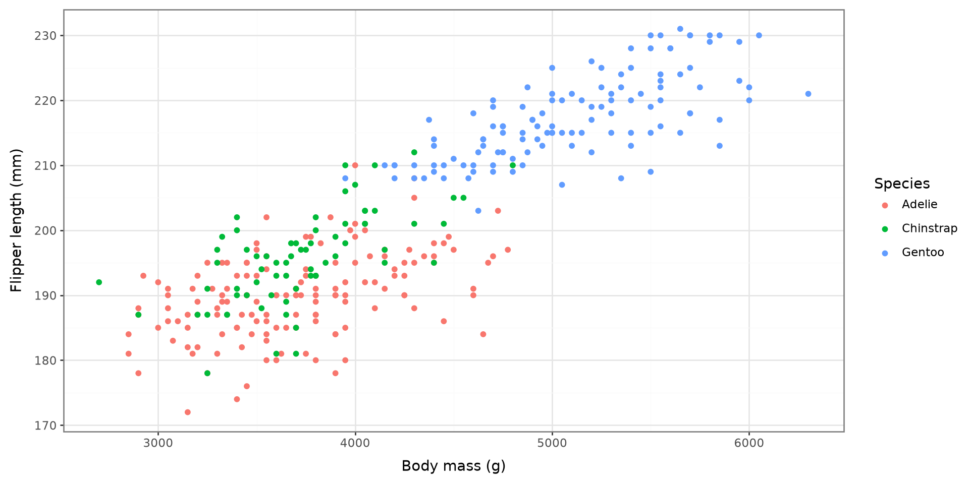
For Now …

Code

(
    ggplot(
        penguins,
        aes(
            x="body_mass_g",
            y="flipper_length_mm",
            color="gentoo",
        ),
    )
    + geom_point()
    + labs(
        x="Body mass (g)",
        y="Flipper length (mm)",
        color="Group",
    )
    + theme_bw()
)

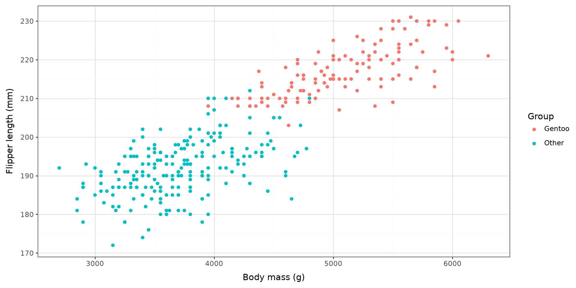
Potential Model

\[ \left(\begin{array}{c} Gentoo \\ Other \end{array}\right) = \boldsymbol X^\mathrm T \boldsymbol \beta \]

Logistic Regression

Logistic Regression is used to model the association between a set of predictors and a binary outcome.

Construct Model

\[ \left(\begin{array}{c} Gentoo \\ Other \end{array}\right) = \boldsymbol X^\mathrm T \boldsymbol \beta \]

Let …

\[ Y = \left\{\begin{array}{cc} 1 & Gentoo \\ 0 & Other \end{array}\right. \]

Construct a Model

\[ P\left(Y = 1\right) = \boldsymbol X^\mathrm T \boldsymbol \beta \]

Construct a Model

\[ P\left(Y = 1\right) = \frac{\exp(\boldsymbol X^\mathrm T \boldsymbol \beta)}{1 + \exp(\boldsymbol X^\mathrm T \boldsymbol \beta)} \]

Construct a Model

\[ \frac{P(Y = 1)}{1-P(Y = 1)} = \exp(\boldsymbol X^\mathrm T \boldsymbol \beta) \]

The Logistic Model

\[ \log\left\{\frac{P(Y = 1)}{1-P(Y = 1)}\right\} = \boldsymbol X^\mathrm T \boldsymbol \beta \]

Odds and Log-Odds

\[ \frac{P(Y = 1)}{1-P(Y = 1)} \]

\[ \log\left\{\frac{P(Y = 1)}{1-P(Y = 1)}\right\} \]

Estimation

Estimation is done by finding the values of \(\boldsymbol \beta\) that maximizes the likelihood function given the data pair \((\boldsymbol X_i, Y_i)\)

\[ L(\boldsymbol \beta) = \prod_{i=1}^n P(Y_i=1)^{Y_i}\left\{1-P(Y_i=1)\right\}^{1-Y_i} \]

Predicting Category

Once the estimates \(\hat \beta\) are obtained, compute:

\[ P\left(Y_i = 1\right) = \frac{\exp(\boldsymbol X_i^\mathrm T \boldsymbol{\hat\beta})}{1 + \exp(\boldsymbol X^\mathrm T \boldsymbol{\hat\beta})} \]

\[ Y_i = \left\{\begin{array}{cc} 1 & P(Y_i =1) \geq 0.5 \\ 0 & Otherwise \end{array}\right. \]

Ordinal Regression

Ordinal regression extends the logistic regression to more than one category (\(J\) Categories) that has a natural order.

An example can be thought of as Grade Levels: A, B, C, D, F

Modeling Ordinal Responses

We can model Ordinal responses using the the proportional odds model and a logit formula:

\[ \mathrm{logit}\{P(Y\leq j|X)\} = \boldsymbol X_{(j)} ^\mathrm T \boldsymbol \beta _{(j)} \]

Linear Model

\[ \boldsymbol X_{(j)}^\mathrm T \boldsymbol \beta_{(j)} = \beta_{0(j)} + \sum^p_{i=1}X_{i}\beta_i \]

Multinomial Regression

Model

\[ \log\left\{\frac{P(Y = k)}{P(Y = \mathrm{REF})}\right\} = \boldsymbol X^\mathrm T \boldsymbol \beta_k \]

\(\mathrm{REF}\) is a reference value to be modeled.

Python Examples

Logistic Regression

model = smf.logit(
    "y ~ x",
    data=data,
).fit(disp=False)

Logistic Regression

logit_result = smf.logit(
    "gentoo_binary ~ flipper_length_mm + body_mass_g",
    data=penguins,
).fit(disp=False)

logit_result.summary()

Logit Regression Results
Dep. Variable:	gentoo_binary	No. Observations:	333
Model:	Logit	Df Residuals:	330
Method:	MLE	Df Model:	2
Date:	Fri, 24 Jul 2026	Pseudo R-squ.:	0.9107
Time:	13:50:00	Log-Likelihood:	-19.375
converged:	True	LL-Null:	-217.08
Covariance Type:	nonrobust	LLR p-value:	1.378e-86

	coef	std err	z	P>\|z\|	[0.025	0.975]
Intercept	-131.6218	30.941	-4.254	0.000	-192.265	-70.978
flipper_length_mm	0.5447	0.138	3.935	0.000	0.273	0.816
body_mass_g	0.0043	0.002	2.616	0.009	0.001	0.008

Possibly complete quasi-separation: A fraction 0.59 of observations can be
perfectly predicted. This might indicate that there is complete
quasi-separation. In this case some parameters will not be identified.

Prediction Logistic Regression

new_penguins = pd.DataFrame(
    {
        "flipper_length_mm": [200, 220],
        "body_mass_g": [4005, 4775],
    }
)

new_penguins.assign(
    predicted_probability_gentoo=logit_result.predict(new_penguins)
)

	flipper_length_mm	body_mass_g	predicted_probability_gentoo
0	200	4005	0.004410
1	220	4775	0.999848

Multinomial Regression

X = sm.add_constant(data[["x"]])
model = sm.MNLogit(data["y"], X)
result = model.fit(method="newton", disp=False)

Multinomial Regression

multinomial_X = sm.add_constant(
    penguins[["body_mass_g", "flipper_length_mm"]]
)
multinomial_model = sm.MNLogit(
    penguins["species"],
    multinomial_X,
)
multinomial_result = multinomial_model.fit(
    method="newton",
    maxiter=200,
    disp=False,
)

Summary

multinomial_result.summary()

MNLogit Regression Results
Dep. Variable:	species	No. Observations:	333
Model:	MNLogit	Df Residuals:	327
Method:	MLE	Df Model:	4
Date:	Fri, 24 Jul 2026	Pseudo R-squ.:	0.6201
Time:	13:50:00	Log-Likelihood:	-133.31
converged:	True	LL-Null:	-350.86
Covariance Type:	nonrobust	LLR p-value:	7.172e-93

species=Chinstrap	coef	std err	z	P>\|z\|	[0.025	0.975]
const	-29.2641	5.340	-5.480	0.000	-39.731	-18.797
body_mass_g	-0.0013	0.000	-2.798	0.005	-0.002	-0.000
flipper_length_mm	0.1720	0.031	5.467	0.000	0.110	0.234
species=Gentoo	coef	std err	z	P>\|z\|	[0.025	0.975]
const	-149.2427	31.696	-4.709	0.000	-211.366	-87.119
body_mass_g	0.0034	0.002	2.055	0.040	0.000	0.007
flipper_length_mm	0.6544	0.144	4.549	0.000	0.372	0.936

Prediction Multinomial Regression

# New observations
new_penguins = pd.DataFrame(
    {
        "body_mass_g": [4005, 4775],
        "flipper_length_mm": [200, 220],
    }
)

# Construct predictors in the same format used to fit the model
new_multinomial_X = sm.add_constant(
    new_penguins[["body_mass_g", "flipper_length_mm"]],
    has_constant="add",
)

# Predicted probability for each species
predicted_probabilities = multinomial_result.predict(
    new_multinomial_X
)

# Replace numeric column names with species names
predicted_probabilities = predicted_probabilities.rename(
    columns=multinomial_model._ynames_map
)

# Choose the species with the largest predicted probability
predicted_species = predicted_probabilities.idxmax(axis=1)

# Combine inputs, probabilities, and final predictions
prediction_results = (
    new_penguins
    .join(predicted_probabilities.add_prefix("prob_"))
    .assign(predicted_species=predicted_species)
)

prediction_results

	body_mass_g	flipper_length_mm	prob_Adelie	prob_Chinstrap	prob_Gentoo	predicted_species
0	4005	200	0.477820	0.517485	0.004695	Chinstrap
1	4775	220	0.000015	0.000192	0.999793	Gentoo