Nonlinear Models

2026-10-13

Notebook

Notebook

Motivating Example

  • Motivating Example

  • Polynomial Functions

  • Step Functions

  • Regression Splines

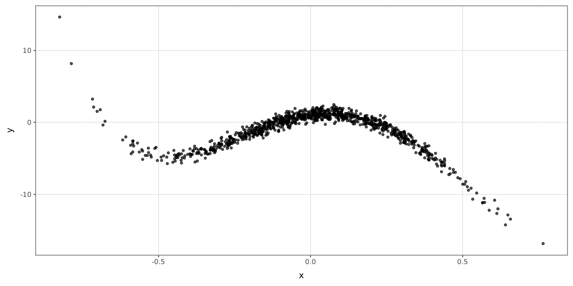
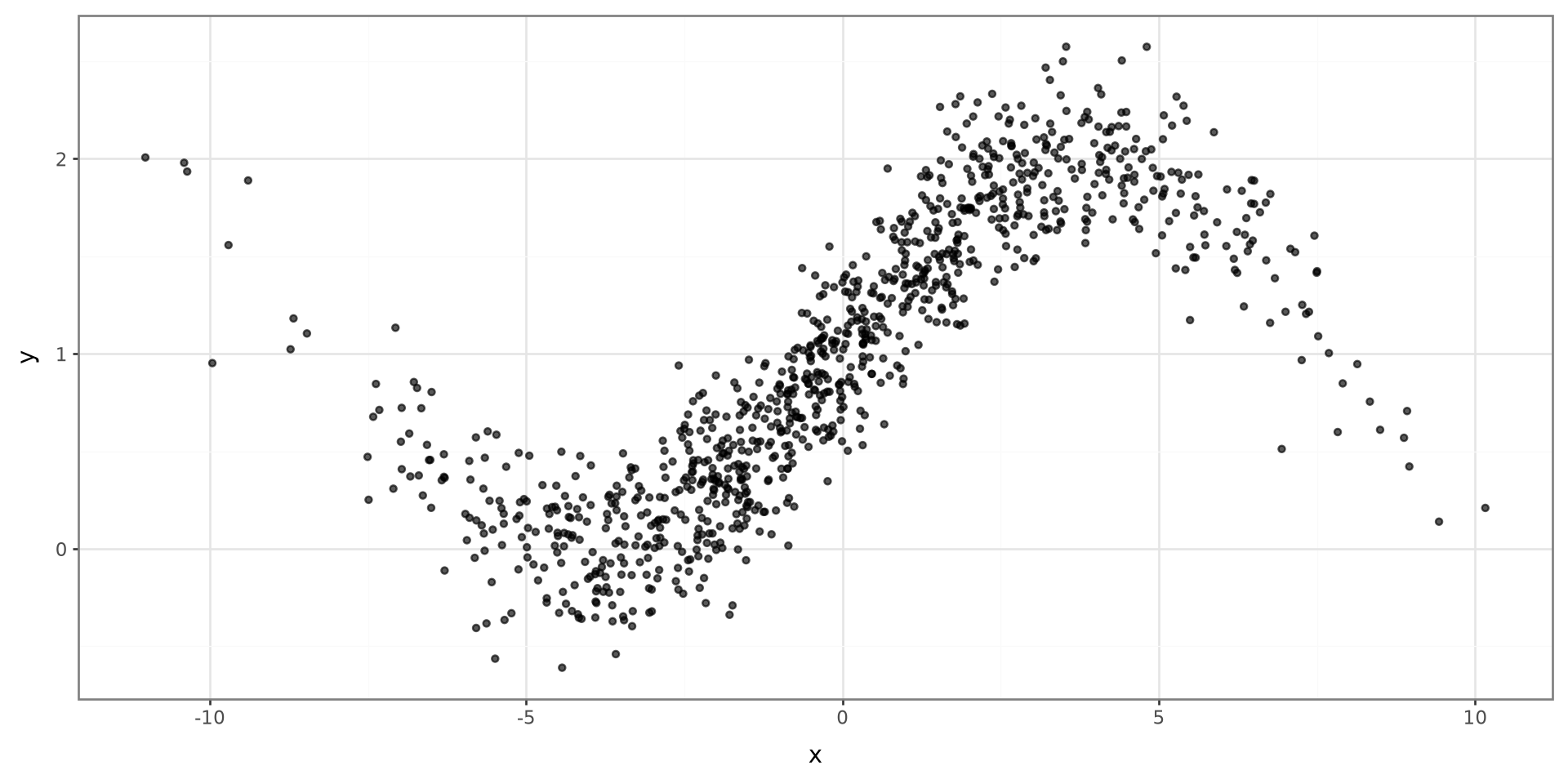
Plot

Show code
(
    ggplot(motivating_polynomial_data, aes(x="x", y="y"))
    + geom_point(size=1.2, alpha=0.65)
    + theme_bw()
)

Plot

Show code
(
    ggplot(motivating_sine_data, aes(x="x", y="y"))
    + geom_point(size=1.2, alpha=0.65)
    + theme_bw()
)

Polynomial Functions

  • Motivating Example

  • Polynomial Functions

  • Step Functions

  • Regression Splines

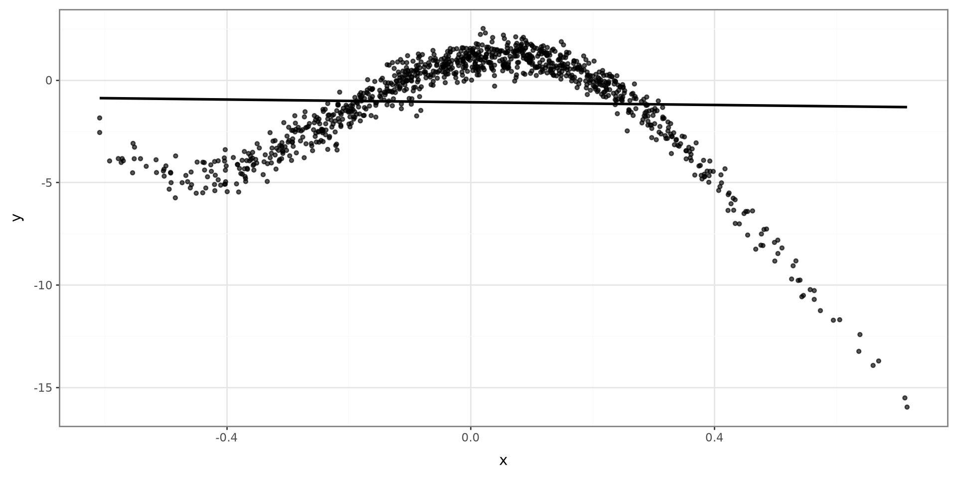
Simple Linear Regression

Simple Linear Regression models the association between one predictor X and an outcome Y:

\[ Y = \beta_0 + \beta_1 X + \varepsilon \]

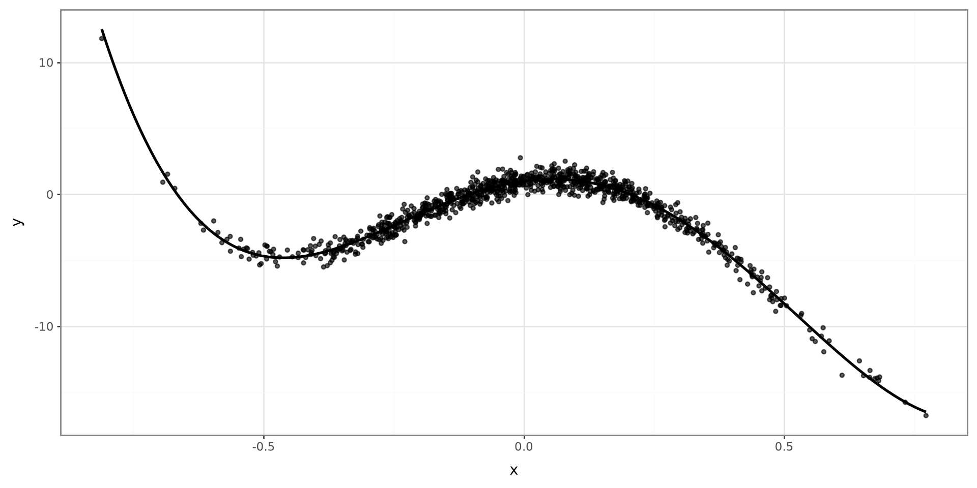
Polynomial Regression

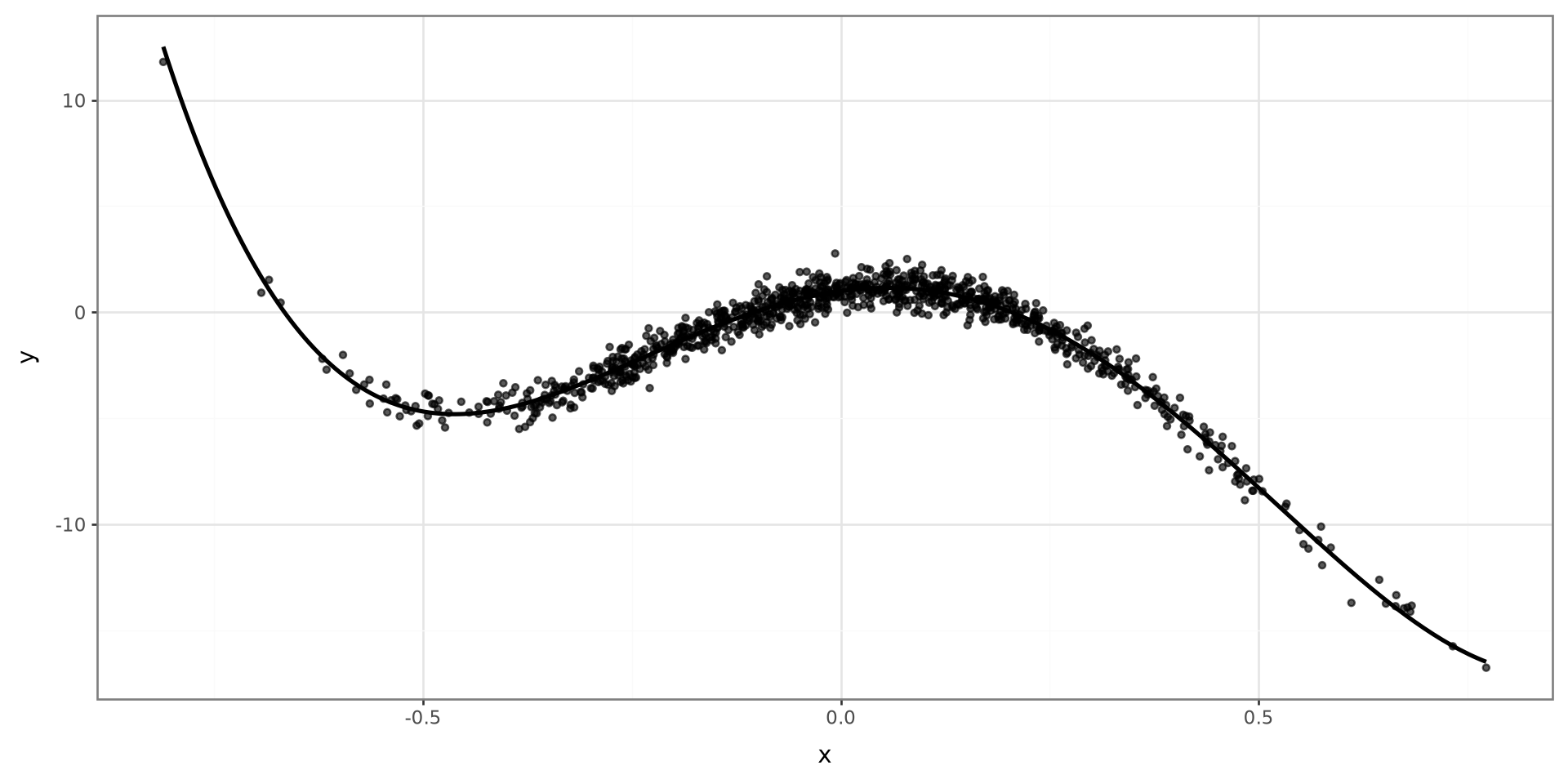
Polynomial Regression models the association between predictor X and outcome Y with a polynomial function. For example, X can be related with Y with a cubic polynomial:

\[ Y = \beta_0 + \beta_1 X + \beta_2 X^2 + \beta_3 X^3 + \varepsilon \]

Finding estimates of \(\boldsymbol \beta\)

The estimates of \(\boldsymbol \beta\) can be found by minimizing the following least squares formula for a given data set:

\[ L(\boldsymbol \beta) = \sum^n_{i=1}(Y_i-\hat Y_i)^2 \]

\[ \hat Y_i = \hat \beta_0 + \hat\beta_1 X_i + \hat\beta_2 X_i^2 + \hat\beta_3 X_i^3 \]

Polynomial Functions in GLMs

Polynomial functions can be utilized in GLMs as well. The model below is for a logistic model:

\[ P(Y=1|X) = \frac{\exp\left\{ \beta_0 + \sum^3_{j=1}\beta_j X^j \right\}}{1 +\exp \left\{ \beta_0 + \sum^3_{j=1}\beta_j X^j\right\}} \]

Fitting a Linear Model

Show code
linear_model = smf.ols("y ~ x", data=linear_fit_data).fit()
linear_grid = pd.DataFrame(
    {"x": np.linspace(linear_fit_data["x"].min(), linear_fit_data["x"].max(), 300)}
)
linear_grid["predicted_y"] = linear_model.predict(linear_grid)

(
    ggplot(linear_fit_data, aes(x="x", y="y"))
    + geom_point(size=1.2, alpha=0.65)
    + geom_line(
        data=linear_grid,
        mapping=aes(x="x", y="predicted_y"),
        inherit_aes=False,
        size=1.1,
    )
    + theme_bw()
)
Fitting a Model

Show code
quartic_model = smf.ols(
    "y ~ x + I(x ** 2) + I(x ** 3) + I(x ** 4)",
    data=quartic_fit_data,
).fit()
quartic_grid = pd.DataFrame(
    {"x": np.linspace(quartic_fit_data["x"].min(), quartic_fit_data["x"].max(), 300)}
)
quartic_grid["predicted_y"] = quartic_model.predict(quartic_grid)

(
    ggplot(quartic_fit_data, aes(x="x", y="y"))
    + geom_point(size=1.2, alpha=0.65)
    + geom_line(
        data=quartic_grid,
        mapping=aes(x="x", y="predicted_y"),
        inherit_aes=False,
        size=1.1,
    )
    + theme_bw()
)
Step Functions

  • Motivating Example

  • Polynomial Functions

  • Step Functions

  • Regression Splines

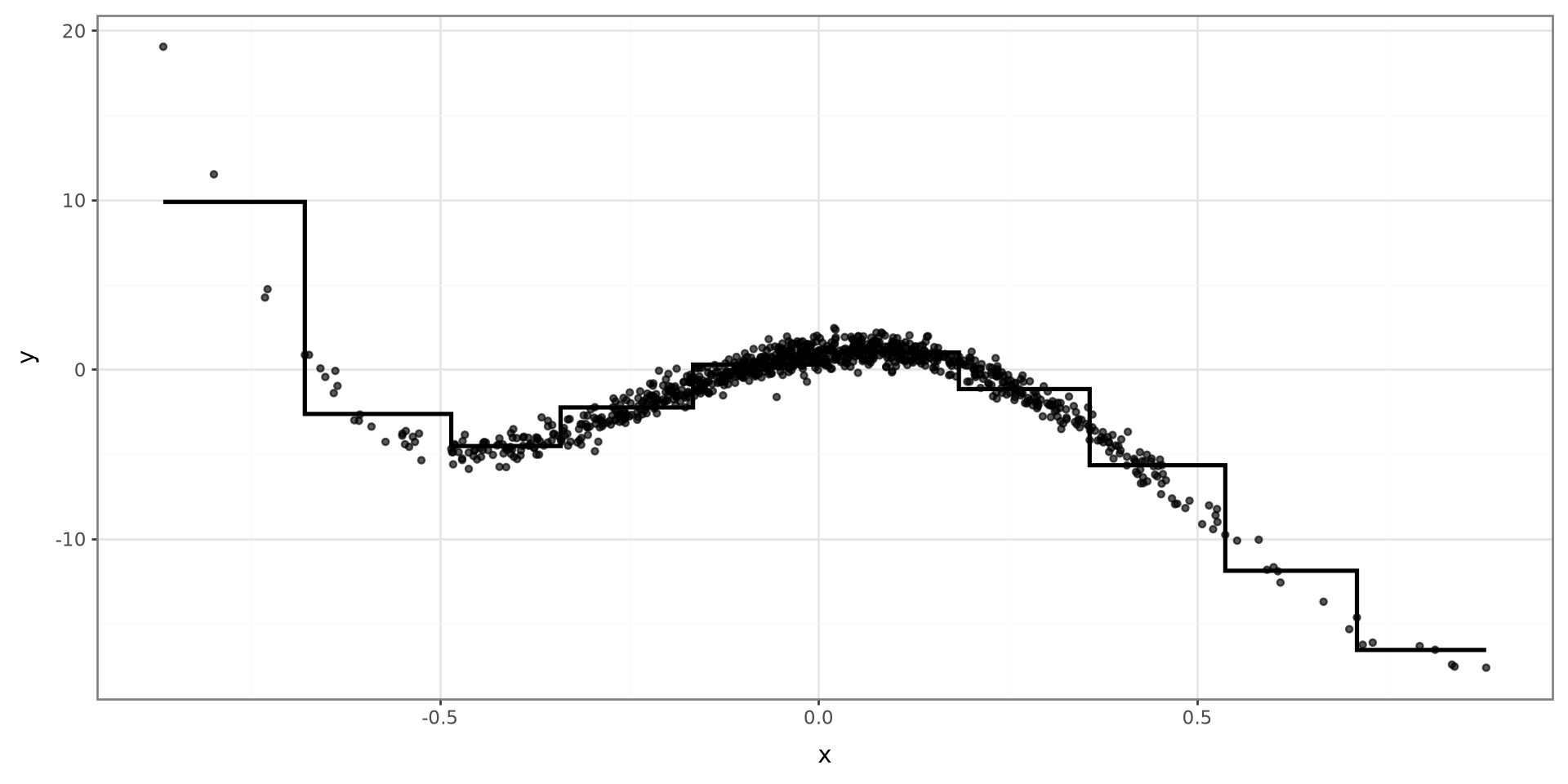
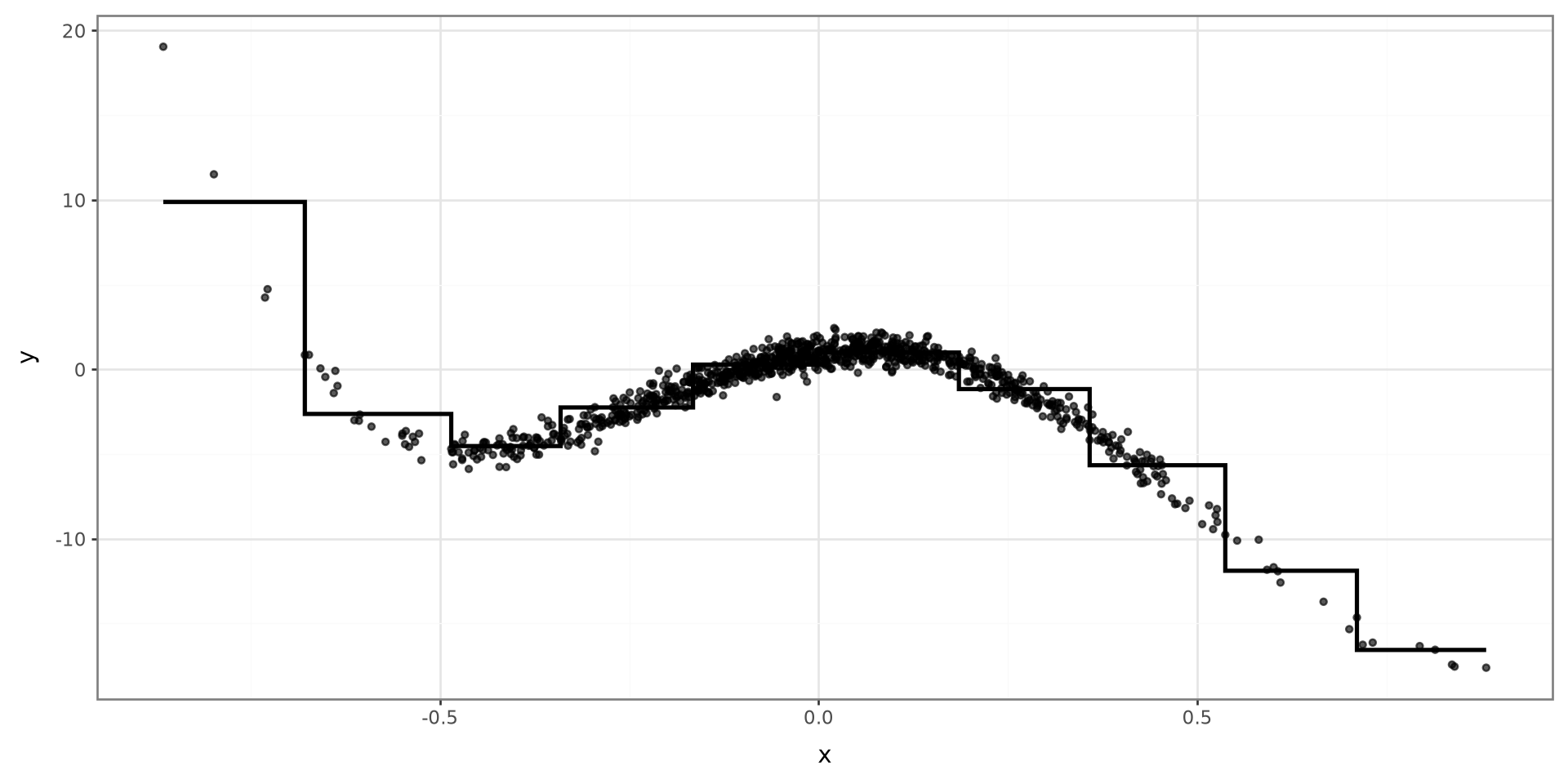
Stepwise Function

Stepwise Function will add horizontal lines to best explain the data at different ranges of X.

Plot

Show code
step_plot = step_plot_data.copy()
step_plot["x_bin"] = pd.cut(step_plot["x"], bins=10, include_lowest=True)
step_plot["predicted_y"] = step_plot.groupby(
    "x_bin",
    observed=True,
)["y"].transform("mean")
step_curve = step_plot.sort_values("x")

(
    ggplot(step_plot, aes(x="x", y="y"))
    + geom_point(size=1.2, alpha=0.65)
    + geom_step(
        data=step_curve,
        mapping=aes(x="x", y="predicted_y"),
        inherit_aes=False,
        size=1.1,
    )
    + theme_bw()
)
Constructing Model

  • Divide the range of X with k different intervals.
  • Create k-1 dummy variables indicating if the value X belongs to the interval or not.
  • Construct a model incorporating all dummy variable and their corresponding coefficient.
  • Find the estimates of the model by minimizing the Least Squares Estimator.

Regression Splines

  • Motivating Example

  • Polynomial Functions

  • Step Functions

  • Regression Splines

Basis Functions

Basis functions model the outcome Y with a set of predefined functions on X:

\[ Y = \beta_0 + \sum^p_{j=1}\beta_jb_j(X) + \varepsilon \]

  • \(\boldsymbol \beta\): Regression Coefficients
  • \(b_j(\cdot)\): basis functions

\(b_j(\cdot)\) is allowed to be any function we define

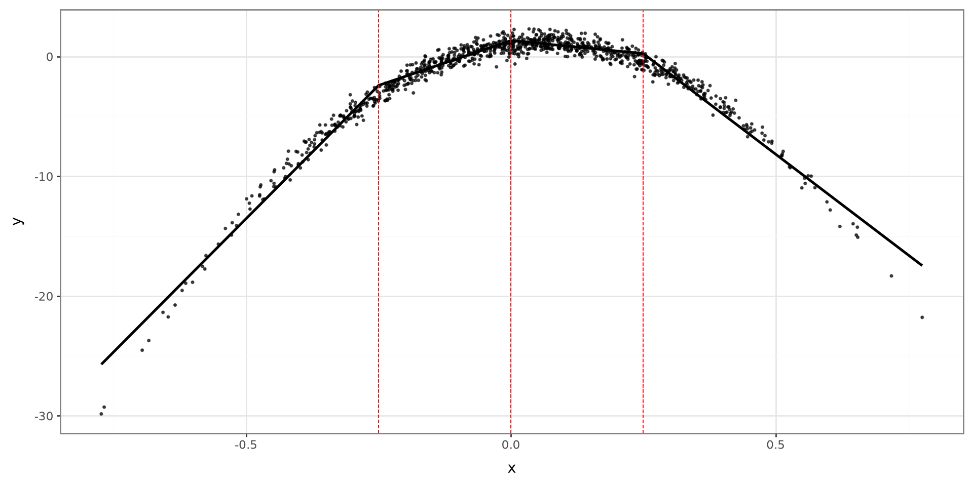
Knots

Show code
knot_model_data = knot_data.assign(
    hinge_0=np.maximum(knot_data["x"], 0)
)
knot_model = smf.ols(
    "y ~ x + hinge_0",
    data=knot_model_data,
).fit()
knot_grid = pd.DataFrame(
    {"x": np.linspace(knot_data["x"].min(), knot_data["x"].max(), 300)}
)
knot_grid["hinge_0"] = np.maximum(knot_grid["x"], 0)
knot_grid["predicted_y"] = knot_model.predict(knot_grid)

(
    ggplot(knot_data, aes(x="x", y="y"))
    + geom_point(size=0.5, alpha=0.65)
    + geom_line(
        data=knot_grid,
        mapping=aes(x="x", y="predicted_y"),
        inherit_aes=False,
        size=1.1,
    )
    + theme_bw()
)
More Knots

Show code
linear_spline_model = smf.ols(
    "y ~ bs(x, knots=(-0.25, 0, 0.25), degree=1)",
    data=more_knots_data,
).fit()
linear_spline_grid = pd.DataFrame(
    {"x": np.linspace(more_knots_data["x"].min(), more_knots_data["x"].max(), 300)}
)
linear_spline_grid["predicted_y"] = linear_spline_model.predict(linear_spline_grid)

(
    ggplot(more_knots_data, aes(x="x", y="y"))
    + geom_point(size=0.5, alpha=0.65)
    + geom_line(
        data=linear_spline_grid,
        mapping=aes(x="x", y="predicted_y"),
        inherit_aes=False,
        size=1.1,
    )
    + geom_vline(
        xintercept=[-0.25, 0, 0.25],
        linetype="dashed",
        size=0.4,
        color="red",
    )
    + theme_bw()
)
Truncated Power Basis Function

Once the number of knots and locations are chosen, a common basis function to utilize is the truncated power function:

\[ h(x,\xi_l) = (x-\xi_l)_+^p = \left\{ \begin{array}{cc} (x-\xi_l)^p & x>\xi_l\\ 0 & \mathrm{Otherwise} \end{array} \right. \]

Spline Function

For \(L\) knots:

\[ Y = \beta_0 + \sum^p_{j=1}x^j\beta_j + \sum_{l=1}^Lh(x, \xi_l)\beta_{p+l} + \varepsilon \]

Spline Functions Constraints

  • When choosing basis functions, we want maintain the following constraints at the location of the knots:
  • Continuous
  • First Differentiable
  • Second Differentiable
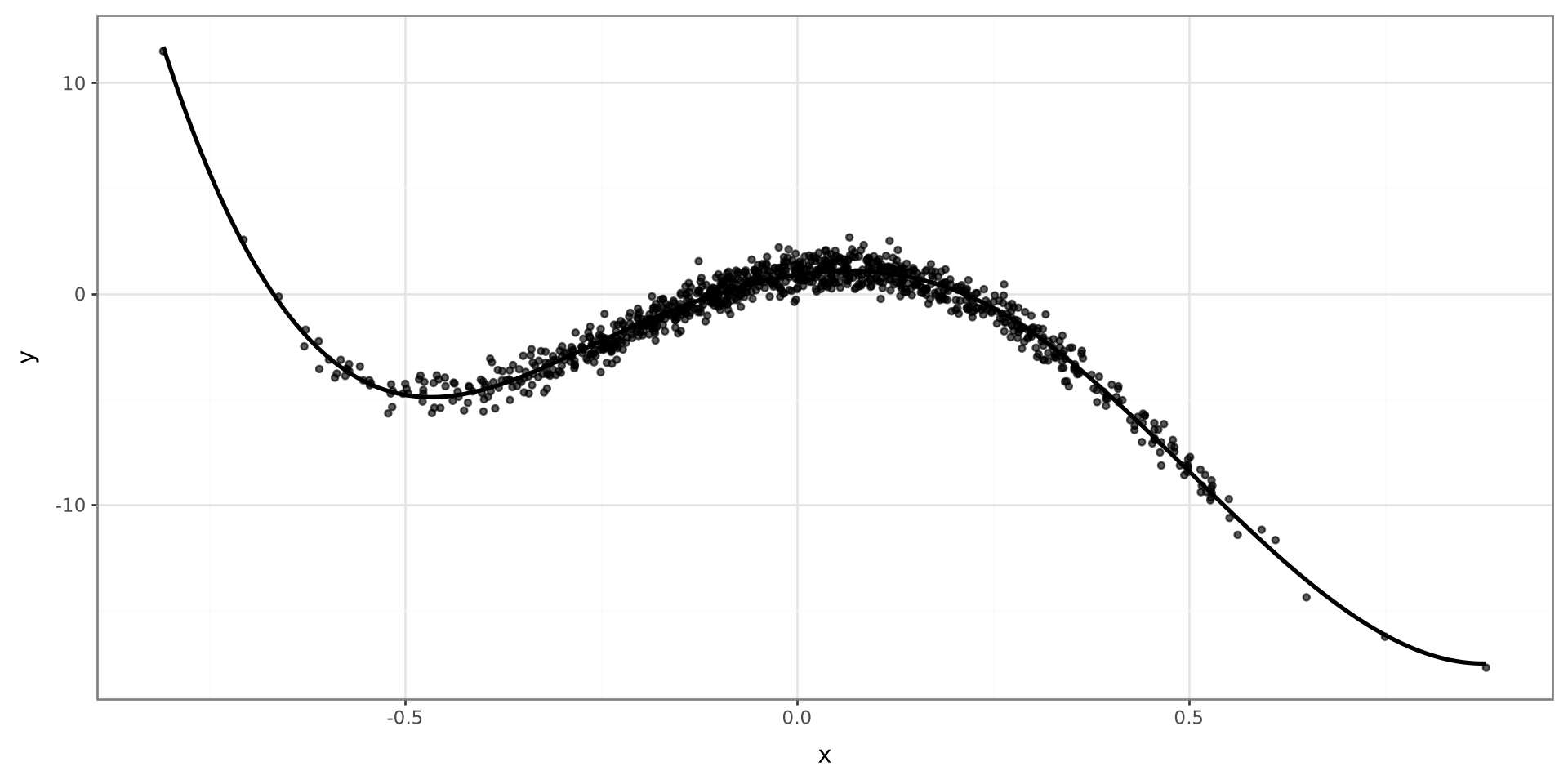
  • A common choice is to use a cubic spline function

Cubic Splines

For \(L\) knots:

\[ Y = \beta_0 + \sum^3_{j=1}x^j\beta_j + \sum_{l=1}^Lh(x, \xi_l)\beta_{3+l} + \varepsilon \]

Natural Cubic Splines

  • Natural splines force the boundary knots to be fitted with simple lines instead of spline functions. The interior knots are fitted with spline functions.
  • The data points outside the interior knots are modeled with lines.

Plot

Show code
cubic_spline_model = smf.ols(
    "y ~ bs(x, knots=(-0.25, 0.25), degree=3)",
    data=cubic_spline_data,
).fit()
cubic_spline_grid = pd.DataFrame(
    {"x": np.linspace(cubic_spline_data["x"].min(), cubic_spline_data["x"].max(), 300)}
)
cubic_spline_grid["predicted_y"] = cubic_spline_model.predict(cubic_spline_grid)

(
    ggplot(cubic_spline_data, aes(x="x", y="y"))
    + geom_point(size=1.2, alpha=0.65)
    + geom_line(
        data=cubic_spline_grid,
        mapping=aes(x="x", y="predicted_y"),
        inherit_aes=False,
        size=1.1,
    )
    + theme_bw()
)
Natural Cubic Splines

Show code
natural_spline_model = smf.ols(
    "y ~ cr(x, knots=(-0.25, 0.25))",
    data=natural_spline_data,
).fit()
natural_spline_grid = pd.DataFrame(
    {"x": np.linspace(natural_spline_data["x"].min(), natural_spline_data["x"].max(), 300)}
)
natural_spline_grid["predicted_y"] = natural_spline_model.predict(natural_spline_grid)

(
    ggplot(natural_spline_data, aes(x="x", y="y"))
    + geom_point(size=1.2, alpha=0.65)
    + geom_line(
        data=natural_spline_grid,
        mapping=aes(x="x", y="predicted_y"),
        inherit_aes=False,
        size=1.1,
    )
    + theme_bw()
)
B-Splines

  • In Python, B-Spline typically refers to the general use of basis functions for models, such as truncated-power, cubic splines, or natural cubic splines.

  • When reading scientific papers, B-Splines typically refers to the implementation of one type of basis function: Cox-de Boer recursion.

  • For this class, we will follow the former and not the latter.