Nonlinear Models

Python Setup

import numpy as np
import pandas as pd
from pickle import TRUE
import statsmodels.formula.api as smf
from plotnine import *
from sklearn.linear_model import LinearRegression
from sklearn.metrics import mean_squared_error, r2_score
from sklearn.preprocessing import PolynomialFeatures


# Use one random-number generator so every simulated dataset is reproducible.
rng = np.random.default_rng(123)


def simulate_quartic_data(n=1000, x_sd=0.25, noise_sd=0.5):
    """Simulate data from the quartic relationship used in the slides."""
    x = rng.normal(loc=0, scale=x_sd, size=n)
    y = (
        1
        + 5.3 * x
        - 45 * x**2
        - 35.5 * x**3
        + 60 * x**4
        + rng.normal(loc=0, scale=noise_sd, size=n)
    )
    return pd.DataFrame({"x": x, "y": y})


def simulate_quadratic_data(n=1000, x_sd=0.25, noise_sd=0.5):
    """Simulate data from the quadratic relationship used for knot examples."""
    x = rng.normal(loc=0, scale=x_sd, size=n)
    y = 1 + 5.3 * x - 45 * x**2 + rng.normal(loc=0, scale=noise_sd, size=n)
    return pd.DataFrame({"x": x, "y": y})


def simulate_sine_data(n=1000, x_sd=3.5, noise_sd=0.25):
    """Simulate data from the sinusoidal relationship used in the slides."""
    x = rng.normal(loc=0, scale=x_sd, size=n)
    y = 1 + np.sin(np.pi * x / 8) + rng.normal(loc=0, scale=noise_sd, size=n)
    return pd.DataFrame({"x": x, "y": y})


# Each object corresponds to one of the original R simulation chunks.
motivating_polynomial_data = simulate_quartic_data()
motivating_sine_data = simulate_sine_data()
linear_fit_data = simulate_quartic_data()
quartic_fit_data = simulate_quartic_data()
polynomial_example_data = simulate_quartic_data()
step_plot_data = simulate_quartic_data()
step_example_data = simulate_quartic_data()
knot_data = simulate_quadratic_data()
more_knots_data = simulate_quadratic_data()
cubic_spline_data = simulate_quartic_data()
natural_spline_data = simulate_quartic_data()
spline_example_data = simulate_quartic_data()

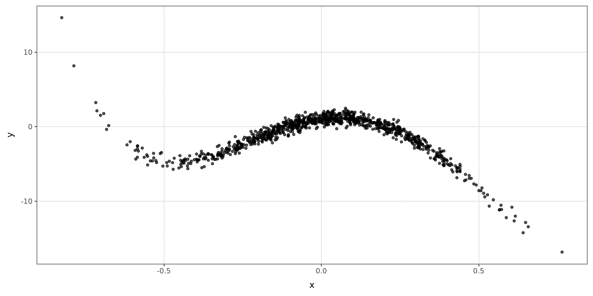
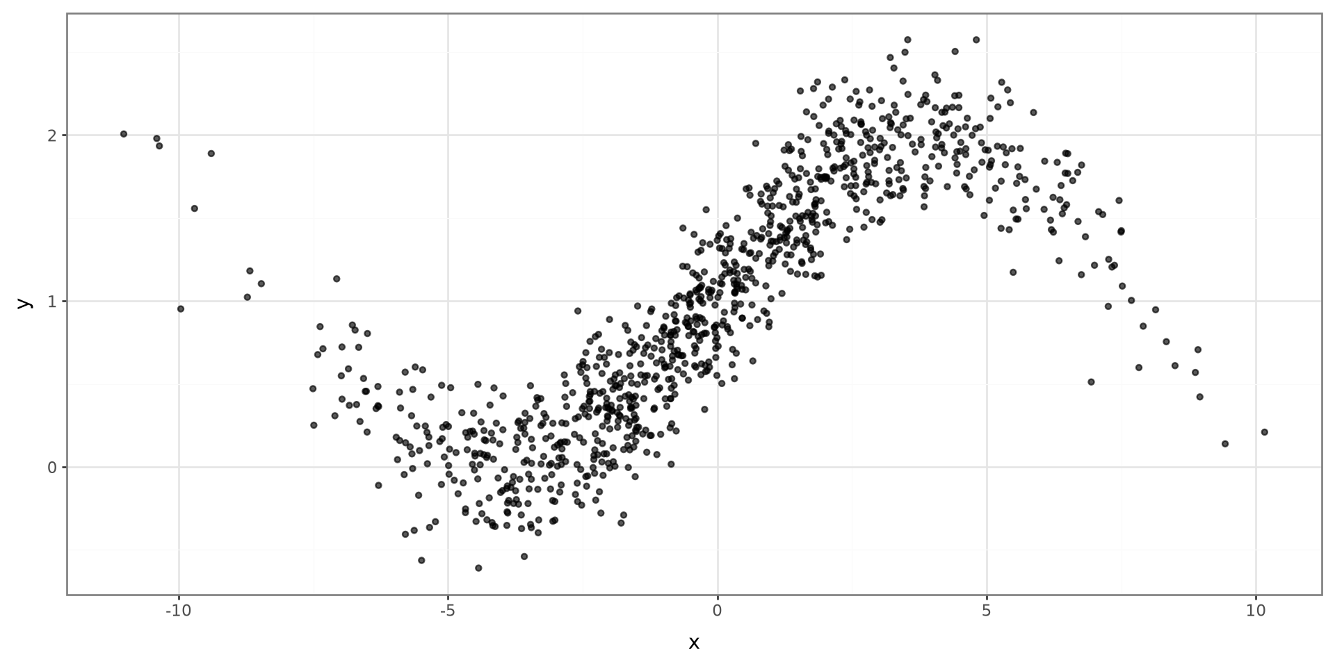
Motivating Example

Plot

(
    ggplot(motivating_polynomial_data, aes(x="x", y="y"))
    + geom_point(size=1.2, alpha=0.65)
    + theme_bw()
)

Plot

(
    ggplot(motivating_sine_data, aes(x="x", y="y"))
    + geom_point(size=1.2, alpha=0.65)
    + theme_bw()
)

Polynomial Functions

Simple Linear Regression

Simple Linear Regression models the association between one predictor X and an outcome Y:

\[ Y = \beta_0 + \beta_1 X + \varepsilon \]

Polynomial Regression

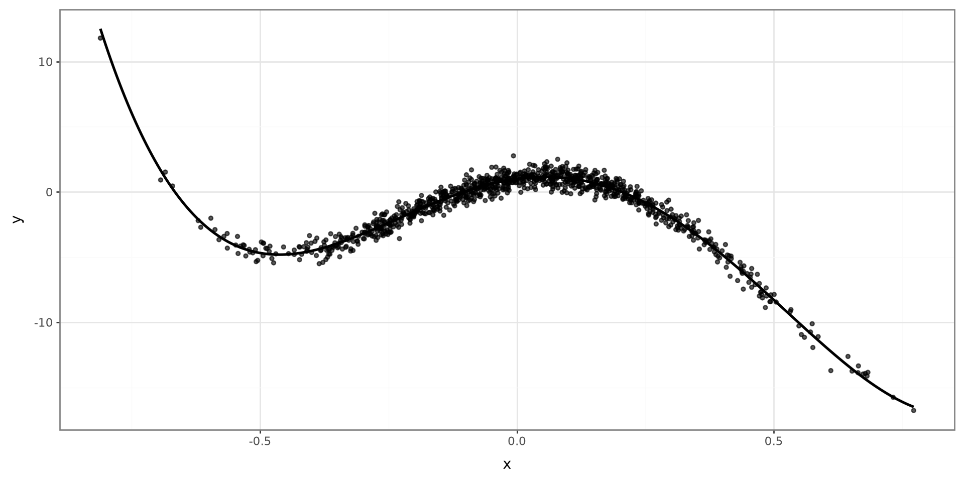
Polynomial Regression models the association between predictor X and outcome Y with a polynomial function. For example, X can be related with Y with a cubic polynomial:

\[ Y = \beta_0 + \beta_1 X + \beta_2 X^2 + \beta_3 X^3 + \varepsilon \]

Finding estimates of \(\boldsymbol \beta\)

The estimates of \(\boldsymbol \beta\) can be found by minimizing the following least squares formula for a given data set:

\[ L(\boldsymbol \beta) = \sum^n_{i=1}(Y_i-\hat Y_i)^2 \]

\[ \hat Y_i = \hat \beta_0 + \hat\beta_1 X_i + \hat\beta_2 X_i^2 + \hat\beta_3 X_i^3 \]

Polynomial Functions in GLMs

Polynomial functions can be utilized in GLMs as well. The model below is for a logistic model:

\[ P(Y=1|X) = \frac{\exp\left\{ \beta_0 + \sum^3_{j=1}\beta_j X^j \right\}}{1 +\exp \left\{ \beta_0 + \sum^3_{j=1}\beta_j X^j\right\}} \]

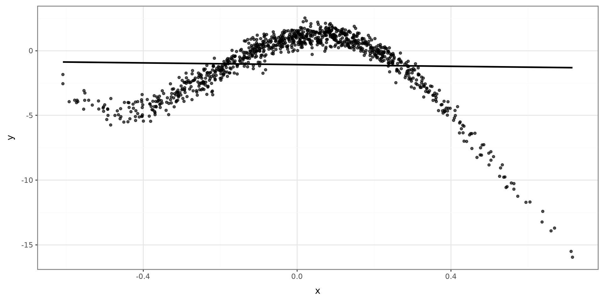
Fitting a Linear Model

linear_model = smf.ols("y ~ x", data=linear_fit_data).fit()
linear_grid = pd.DataFrame(
    {"x": np.linspace(linear_fit_data["x"].min(), linear_fit_data["x"].max(), 300)}
)
linear_grid["predicted_y"] = linear_model.predict(linear_grid)

(
    ggplot(linear_fit_data, aes(x="x", y="y"))
    + geom_point(size=1.2, alpha=0.65)
    + geom_line(
        data=linear_grid,
        mapping=aes(x="x", y="predicted_y"),
        inherit_aes=False,
        size=1.1,
    )
    + theme_bw()
)

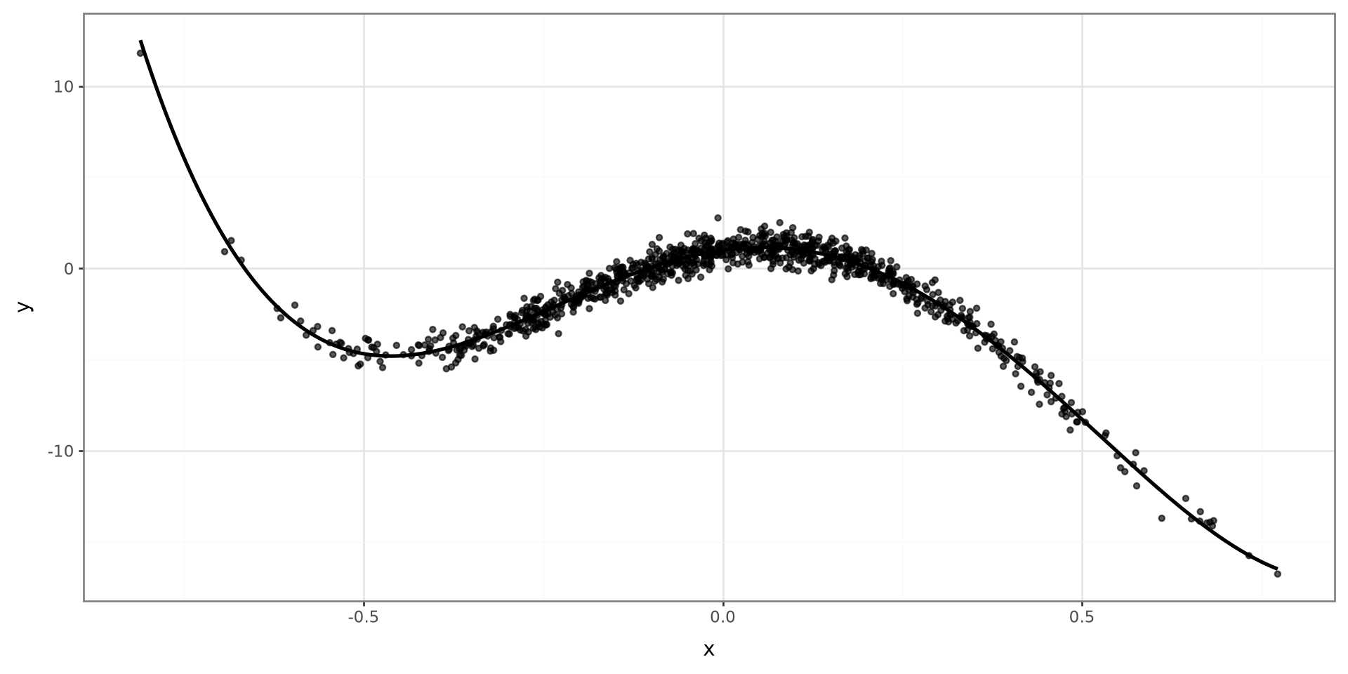
Fitting a Model

quartic_model = smf.ols(
    "y ~ x + I(x ** 2) + I(x ** 3) + I(x ** 4)",
    data=quartic_fit_data,
).fit()
quartic_grid = pd.DataFrame(
    {"x": np.linspace(quartic_fit_data["x"].min(), quartic_fit_data["x"].max(), 300)}
)
quartic_grid["predicted_y"] = quartic_model.predict(quartic_grid)

(
    ggplot(quartic_fit_data, aes(x="x", y="y"))
    + geom_point(size=1.2, alpha=0.65)
    + geom_line(
        data=quartic_grid,
        mapping=aes(x="x", y="predicted_y"),
        inherit_aes=False,
        size=1.1,
    )
    + theme_bw()
)

Polynomial Functions in Python (Alternative)

polynomial = PolynomialFeatures(degree=p, include_bias=False)
X_polynomial = polynomial.fit_transform(data[["x"]])
model = LinearRegression().fit(X_polynomial, data["y"])

Example Plot

quartic_transform = PolynomialFeatures(degree=4, include_bias=True)
X_quartic = quartic_transform.fit_transform(quartic_fit_data[["x"]])
quartic_model_2 = LinearRegression().fit(X_quartic, quartic_fit_data["y"])



quartic_grid_2 = pd.DataFrame(
    {"x": np.linspace(quartic_fit_data["x"].min(), quartic_fit_data["x"].max(), 300)}
)

quartic_grid_2_transform = quartic_transform.fit_transform(quartic_grid_2[["x"]])

quartic_grid_2["predicted_y"] = quartic_model_2.predict(quartic_grid_2_transform)

(
    ggplot(quartic_fit_data, aes(x="x", y="y"))
    + geom_point(size=1.2, alpha=0.65)
    + geom_line(
        data=quartic_grid_2,
        mapping=aes(x="x", y="predicted_y"),
        inherit_aes=False,
        size=1.1,
    )
    + theme_bw()
)

Individual Terms in Python

model = smf.ols(
    "y ~ I(x ** 3)",
    data=data,
).fit()

Example

Using polynomial_example_data from the setup chunk, fit quadratic, cubic, and quartic models. Compute the mean squared error and \(R^2\) for each model.

polynomial_example_data.head()

	x	y
0	-0.515061	-4.371471
1	-0.052983	0.533842
2	0.317888	-2.973370
3	-0.133988	-1.003931
4	-0.122652	-1.011330

Step Functions

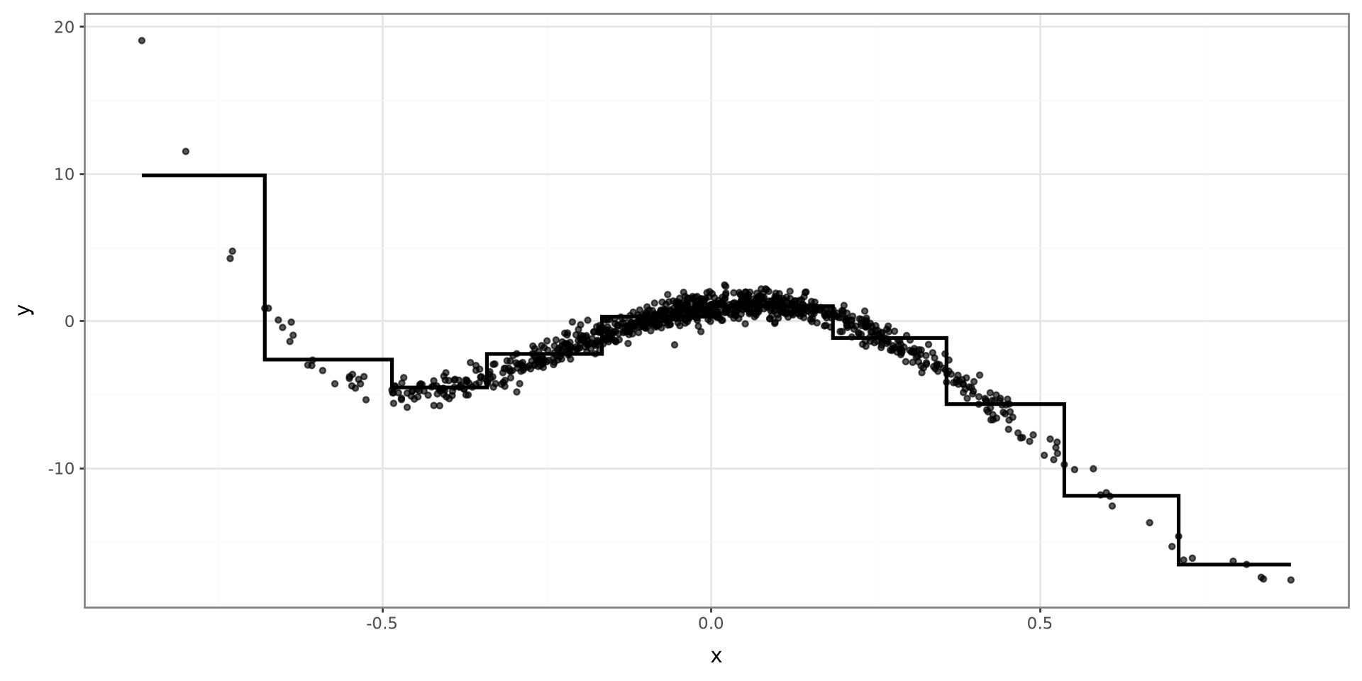
Stepwise Function

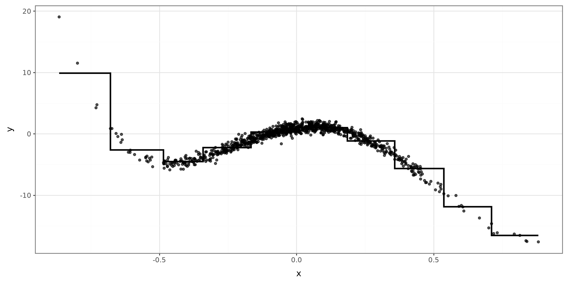
Stepwise Function will add horizontal lines to best explain the data at different ranges of X.

Plot

step_plot = step_plot_data.copy()
step_plot["x_bin"] = pd.cut(step_plot["x"], bins=10, include_lowest=True)
step_plot["predicted_y"] = step_plot.groupby(
    "x_bin",
    observed=True,
)["y"].transform("mean")
step_curve = step_plot.sort_values("x")

(
    ggplot(step_plot, aes(x="x", y="y"))
    + geom_point(size=1.2, alpha=0.65)
    + geom_step(
        data=step_curve,
        mapping=aes(x="x", y="predicted_y"),
        inherit_aes=False,
        size=1.1,
    )
    + theme_bw()
)

Constructing Model

• Divide the range of X with k different intervals.
• Create k-1 dummy variables indicating if the value X belongs to the interval or not.
• Construct a model incorporating all dummy variable and their corresponding coefficient.
• Find the estimates of the model by minimizing the Least Squares Estimator.

Step Functions in Python

step_data = data.assign(
    x_bin=pd.cut(data["x"], bins=10, include_lowest=True)
)
step_model = smf.ols(
    "y ~ C(x_bin)",
    data=step_data,
).fit()

Example

Using step_example_data from the setup chunk, fit step-regression models with 10, 20, and 30 steps. Compute the mean squared error and \(R^2\) for each model.

step_example_data.head()

	x	y
0	0.380932	-4.140677
1	0.496003	-9.234772
2	0.054014	1.920086
3	-0.128841	0.189173
4	0.454639	-6.080184

Regression Splines

Basis Functions

Basis functions model the outcome Y with a set of predefined functions on X:

\[ Y = \beta_0 + \sum^p_{j=1}\beta_jb_j(X) + \varepsilon \]

• \(\boldsymbol \beta\): Regression Coefficients
• \(b_j(\cdot)\): basis functions

\(b_j(\cdot)\) is allowed to be any function we define

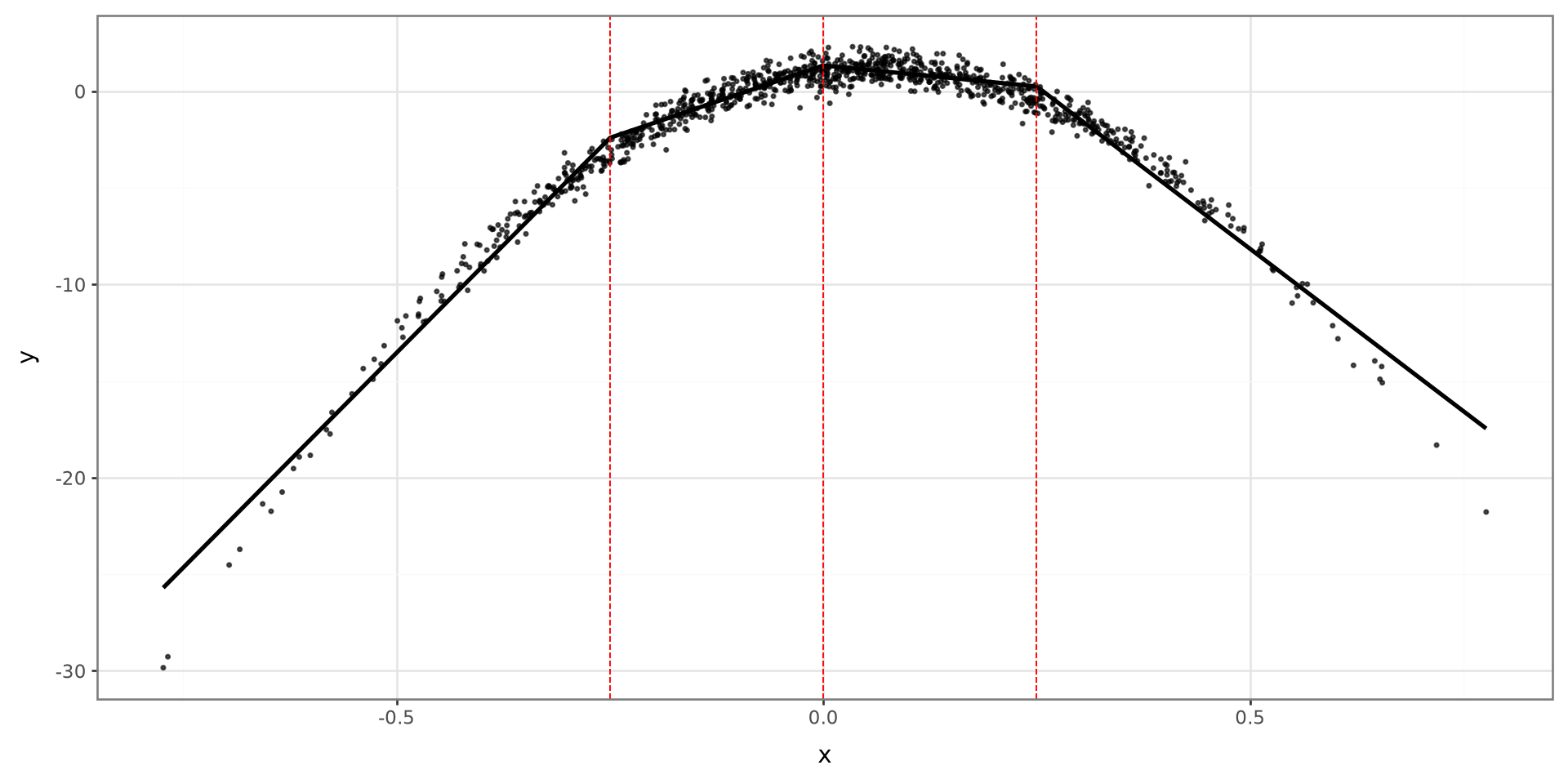
Knots

knot_model_data = knot_data.assign(
    hinge_0=np.maximum(knot_data["x"], 0)
)
knot_model = smf.ols(
    "y ~ x + hinge_0",
    data=knot_model_data,
).fit()
knot_grid = pd.DataFrame(
    {"x": np.linspace(knot_data["x"].min(), knot_data["x"].max(), 300)}
)
knot_grid["hinge_0"] = np.maximum(knot_grid["x"], 0)
knot_grid["predicted_y"] = knot_model.predict(knot_grid)

(
    ggplot(knot_data, aes(x="x", y="y"))
    + geom_point(size=0.5, alpha=0.65)
    + geom_line(
        data=knot_grid,
        mapping=aes(x="x", y="predicted_y"),
        inherit_aes=False,
        size=1.1,
    )
    + theme_bw()
)

More Knots

linear_spline_model = smf.ols(
    "y ~ bs(x, knots=(-0.25, 0, 0.25), degree=1)",
    data=more_knots_data,
).fit()
linear_spline_grid = pd.DataFrame(
    {"x": np.linspace(more_knots_data["x"].min(), more_knots_data["x"].max(), 300)}
)
linear_spline_grid["predicted_y"] = linear_spline_model.predict(linear_spline_grid)

(
    ggplot(more_knots_data, aes(x="x", y="y"))
    + geom_point(size=0.5, alpha=0.65)
    + geom_line(
        data=linear_spline_grid,
        mapping=aes(x="x", y="predicted_y"),
        inherit_aes=False,
        size=1.1,
    )
    + geom_vline(
        xintercept=[-0.25, 0, 0.25],
        linetype="dashed",
        size=0.4,
        color="red",
    )
    + theme_bw()
)

Truncated Power Basis Function

Once the number of knots and locations are chosen, a common basis function to utilize is the truncated power function:

\[ h(x,\xi_l) = (x-\xi_l)_+^p = \left\{ \begin{array}{cc} (x-\xi_l)^p & x>\xi_l\\ 0 & \mathrm{Otherwise} \end{array} \right. \]

Spline Function

For \(L\) knots:

\[ Y = \beta_0 + \sum^p_{j=1}x^j\beta_j + \sum_{l=1}^Lh(x, \xi_l)\beta_{p+l} + \varepsilon \]

Spline Functions Constraints

When choosing basis functions, we want maintain the following constraints at the location of the knots:

• Continuous
• First Differentiable
• Second Differentiable

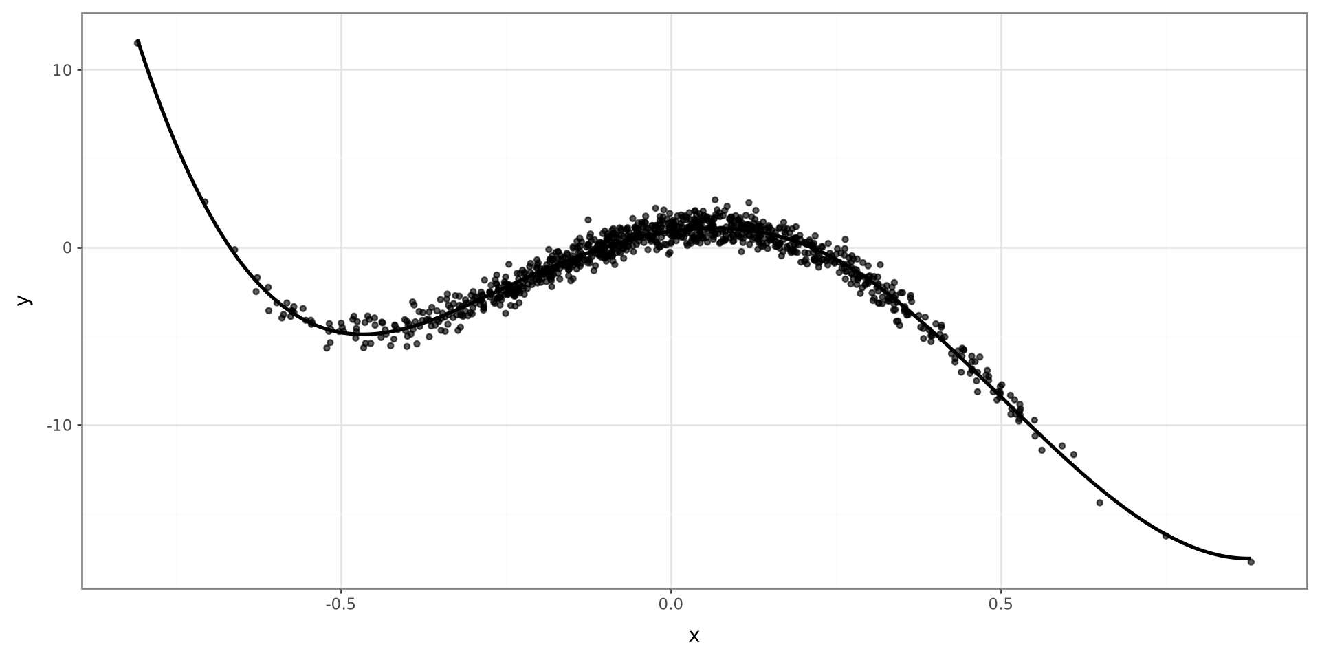
A common choice is to use a cubic spline function

Cubic Splines

For \(L\) knots:

\[ Y = \beta_0 + \sum^3_{j=1}x^j\beta_j + \sum_{l=1}^Lh(x, \xi_l)\beta_{3+l} + \varepsilon \]

Natural Cubic Splines

Natural splines force the boundary knots to be fitted with simple lines instead of spline functions. The interior knots are fitted with spline functions.

Plot

cubic_spline_model = smf.ols(
    "y ~ bs(x, knots=(-0.25, 0.25), degree=3)",
    data=cubic_spline_data,
).fit()
cubic_spline_grid = pd.DataFrame(
    {"x": np.linspace(cubic_spline_data["x"].min(), cubic_spline_data["x"].max(), 300)}
)
cubic_spline_grid["predicted_y"] = cubic_spline_model.predict(cubic_spline_grid)

(
    ggplot(cubic_spline_data, aes(x="x", y="y"))
    + geom_point(size=1.2, alpha=0.65)
    + geom_line(
        data=cubic_spline_grid,
        mapping=aes(x="x", y="predicted_y"),
        inherit_aes=False,
        size=1.1,
    )
    + theme_bw()
)

Natural Cubic Splines

natural_spline_model = smf.ols(
    "y ~ cr(x, knots=(-0.25, 0.25))",
    data=natural_spline_data,
).fit()
natural_spline_grid = pd.DataFrame(
    {"x": np.linspace(natural_spline_data["x"].min(), natural_spline_data["x"].max(), 300)}
)
natural_spline_grid["predicted_y"] = natural_spline_model.predict(natural_spline_grid)

(
    ggplot(natural_spline_data, aes(x="x", y="y"))
    + geom_point(size=1.2, alpha=0.65)
    + geom_line(
        data=natural_spline_grid,
        mapping=aes(x="x", y="predicted_y"),
        inherit_aes=False,
        size=1.1,
    )
    + theme_bw()
)

Cubic Splines in Python

Patsy’s bs() transform constructs a B-spline basis that can be used in a statsmodels formula. Specify the knot locations; a cubic basis uses degree=3.

cubic_spline_model = smf.ols(
    "y ~ bs(x, knots=(...), degree=3)",
    data=data,
).fit()

Natural Cubic Splines in Python

Patsy’s cr() transform constructs a natural cubic regression-spline basis. Specify the knot locations in the model formula.

natural_spline_model = smf.ols(
    "y ~ cr(x, knots=(...))",
    data=data,
).fit()

Example

Using spline_example_data from the setup chunk, fit regression models using cubic splines and natural cubic splines. Choose an appropriate number and location of knots. Compute the mean squared error and \(R^2\) for each model.

spline_example_data.head()

	x	y
0	0.197223	0.013993
1	0.042517	1.922424
2	-0.343305	-4.065611
3	0.060269	0.700677
4	0.443878	-6.708105