Generalized Additive Models

Python Setup

Code

import warnings

import numpy as np
import pandas as pd
import statsmodels.api as sm
from plotnine import (
    aes,
    geom_line,
    geom_point,
    geom_vline,
    ggplot,
    labs,
    theme_bw,
)
from plotnine.data import mtcars
from scipy.interpolate import make_smoothing_spline
from scipy.special import expit
from sklearn.metrics import mean_squared_error
from sklearn.model_selection import KFold
from statsmodels.gam.api import BSplines, GLMGam

warnings.filterwarnings("ignore")

rng = np.random.default_rng(123)


def simulate_polynomial_data(rng, n=1000, x_sd=0.25, error_sd=0.5):
    """Simulate the polynomial relationship used throughout the slides."""
    x = rng.normal(loc=0, scale=x_sd, size=n)
    y = (
        1
        + 5.3 * x
        - 45 * x**2
        - 35.5 * x**3
        + 60 * x**4
        + rng.normal(loc=0, scale=error_sd, size=n)
    )
    return pd.DataFrame({"x": x, "y": y})


# Data for the motivating examples
polynomial_plot_data = simulate_polynomial_data(rng)

x_sine = rng.normal(loc=0, scale=3.5, size=1000)
y_sine = 1 + np.sin(np.pi * x_sine / 8) + rng.normal(
    loc=0,
    scale=0.25,
    size=1000,
)
sinusoidal_plot_data = pd.DataFrame({"x": x_sine, "y": y_sine})

# Separate simulated datasets for the spline and local-regression examples
spline_example_data = simulate_polynomial_data(rng)

# Data for the GAM examples
mtcars_data = mtcars.copy()

x_gam = rng.normal(loc=0, scale=1, size=1000)
y_gam = rng.normal(loc=4, scale=1, size=1000)
mu_gam = np.exp(-2 + expit(x_gam) + np.sqrt(y_gam + 15))
z_gam = rng.poisson(mu_gam)
poisson_gam_data = pd.DataFrame(
    {"x": x_gam, "y": y_gam, "mu": mu_gam, "z": z_gam}
)

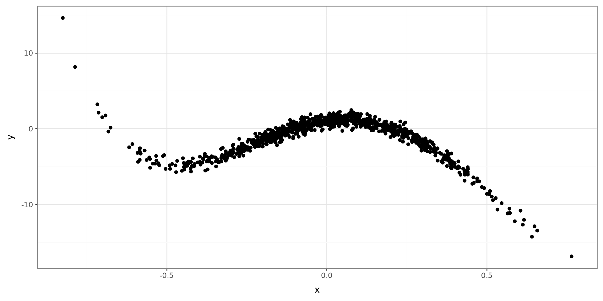
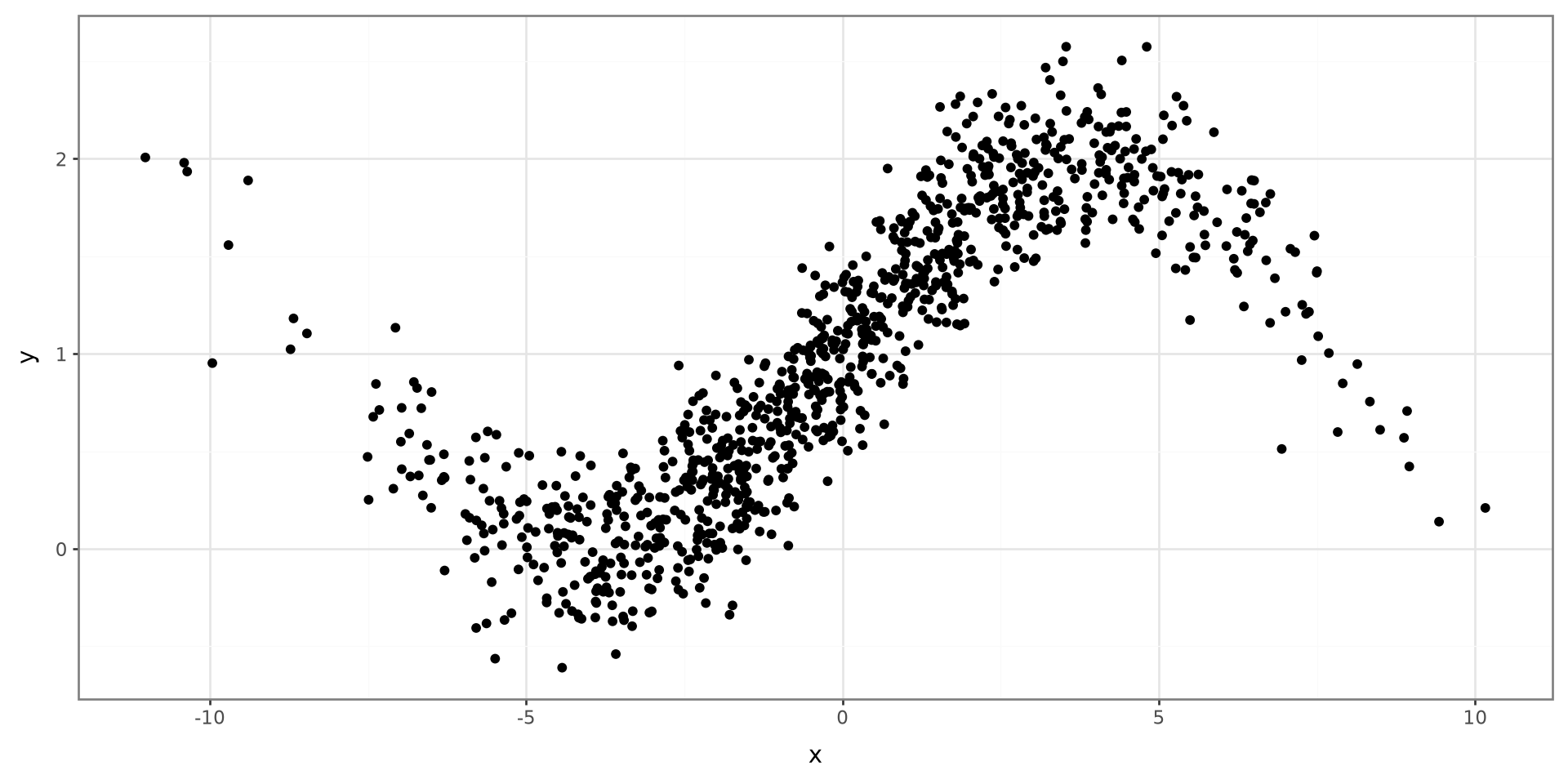
Motivating Example

Plot

Code

(
    ggplot(polynomial_plot_data, aes(x="x", y="y"))
    + geom_point()
    + theme_bw()
)

Plot

Code

(
    ggplot(sinusoidal_plot_data, aes(x="x", y="y"))
    + geom_point()
    + theme_bw()
)

Smoothing Splines

Regression Splines

For \(L\) knots:

\[ Y = \beta_0 + \sum^p_{j=1}x^j\beta_j + \sum_{l=1}^L \beta_{p+l}(x - \xi_l)^p_+ + \varepsilon \]

Issues with Regression Splines

Must specify a correct number of knots
Must specify the correct location of knots
Must specify the degree p

Solutions

Use \(p=3\), performs the best
Implement a penalty term

Smooting Parameter

A smoothing (penalty) parameter will allow us to specify a large number of knots to grid up the range of X.

The smoothing parameter will will force the effect of certain knots to zero that are not relevant.

As long as we choose a high number of knots (20-30), it will properly model the data without the worry of overfitting.

The smoothing parameter can be estimated by using a cross-validation approach and identifying the which values lowers the MSE.

Likelihood Function

\[ \sum^n_{i=1}\{Y_i-g(X_i)\}^2 + \lambda\int g^{\prime\prime}(t)^2dt \]

\(g(\cdot)\): function used to model data (using cubic splines)
\(\lambda\): smoothing parameter

Smoothing Splines in Python

spline_model, best_lambda, mse, cv_results = fit_smoothing_spline_cv(
    data=spline_example_data,
    lambda_grid=np.logspace(-8, 1, 25),
    n_splits=10,
)

Example

Fit a smoothing spline model with the following simulated data. Search through the help documentation to print out \(\lambda\). What is the MSE?

The simulated data are loaded in the setup chunk as spline_example_data.

Code

spline_example_data.head()

	x	y
0	0.035227	1.858924
1	0.359061	-3.492532
2	0.504016	-8.470404
3	-0.328614	-3.795633
4	-0.039906	0.950307

Generalized Additive Models

GAM

Generalized Additive Models extends the nonparametric models to include more than one predictor to explain the outcome Y.

GAM

\[ Y = \beta_0 + f_1(X_1) + f_2(X_2) + \cdots + f_k(X_k) + \varepsilon \]

\[ Y = \beta_0 + \sum^k_{j=1} f_j(X_j) +\varepsilon \]

GAM Estimation

Each \(\hat f_j\) can be estimated using an approach mentioned before.

\[ \hat Y = \hat \beta_0 + \sum^k_{j=1} \hat f_j(X_j) \]

Each \(hat f_j\) can be estimated differently from other predictor functions.

GAMs for Non-Normal Variables

GAMs can be extended to model outcome variables that do not follow a normal distribution.

\[ g(\hat Y) = \hat \beta_0 + \sum^k_{j=1} \hat f_j(X_j) \]

GAMs in Python

The statsmodels package provides functions for fitting GAMs with multiple predictor variables.

smooth_predictors = data[["x_1", "x_2"]]
linear_predictors = sm.add_constant(data[["x_3"]])

spline_basis = BSplines(
    smooth_predictors,
    df=[8, 8],
    degree=[3, 3],
)

gam_model = GLMGam(
    data["y"],
    exog=linear_predictors,
    smoother=spline_basis,
    family=sm.families.Gaussian(),
).fit()

Example

Using mtcars_data, fit a GAM with mpg as an outcome variable with 3 or 4 predictors. Use different types of functions to model the predictors.

Example

Fit the data using the simulated data below:

The simulated data are loaded in the setup chunk as poisson_gam_data.

poisson_gam_data.head()

	x	y	mu	z
0	-1.413310	5.118738	14.601206	11
1	-0.071873	2.673188	14.672697	20
2	0.058539	4.634443	19.024119	17
3	-0.499851	4.974019	17.232651	19
4	0.880485	3.423580	20.069323	18